6. Example 6: Three-bar Truss Design
Example of solving the constrained engineering optimization problem “Three-bar truss design” using NEORL with the BAT, GWO, and MFO algorithms.
6.1. Summary
Algorithms: BAT, GWO, MFO
Type: Continuous, Single-objective, Constrained
Field: Structural Engineering
6.2. Problem Description
The Three-bar truss design is an engineering optimization problem with the objective to evaluate the optimal cross sectional areas \(A_1 = A_3 = x_1\) and \(A_2 = x_2\) such that the volume of the statically loaded truss structure is minimized accounting for stress \((\sigma)\) constraints. The figure below shows the dimensions of the three-bar truss structure.
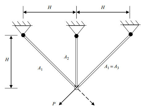
The equation for the volume of the truss structure is
subject to 3 constraints
where \(0 \leq x_1 \leq 1\), \(0 \leq x_2 \leq 1\), \(H = 100 cm\), \(P = 2 KN/cm^2\), and \(\sigma = 2 KN/cm^2\).
6.3. NEORL script
#---------------------------------
# Import packages
#---------------------------------
import numpy as np
from math import cos, pi, exp, e, sqrt
import matplotlib.pyplot as plt
from neorl import BAT, GWO, MFO
#---------------------------------
# Fitness function
#---------------------------------
def TBT(individual):
"""Three-bar truss Design
"""
x1 = individual[0]
x2 = individual[1]
y = (2*sqrt(2)*x1 + x2) * 100
#Constraints
if x1 <= 0:
g = [1,1,1]
else:
g1 = (sqrt(2)*x1+x2)/(sqrt(2)*x1**2 + 2*x1*x2) * 2 - 2
g2 = x2/(sqrt(2)*x1**2 + 2*x1*x2) * 2 - 2
g3 = 1/(x1 + sqrt(2)*x2) * 2 - 2
g = [g1,g2,g3]
g_round=np.round(np.array(g),6)
w1=100
w2=100
phi=sum(max(item,0) for item in g_round)
viol=sum(float(num) > 0 for num in g_round)
return y + w1*phi + w2*viol
#---------------------------------
# Parameter space
#---------------------------------
nx = 2
BOUNDS = {}
for i in range(1, nx+1):
BOUNDS['x'+str(i)]=['float', 0, 1]
#---------------------------------
# BAT
#---------------------------------
bat=BAT(mode='min', bounds=BOUNDS, fit=TBT, nbats=10, fmin = 0 , fmax = 1, A=0.5, r0=0.5, levy = True, seed = 1, ncores=1)
bat_x, bat_y, bat_hist=bat.evolute(ngen=100, verbose=1)
#---------------------------------
# GWO
#---------------------------------
gwo=GWO(mode='min', fit=TBT, bounds=BOUNDS, nwolves=10, ncores=1, seed=1)
gwo_x, gwo_y, gwo_hist=gwo.evolute(ngen=100, verbose=1)
#---------------------------------
# MFO
#---------------------------------
mfo=MFO(mode='min', bounds=BOUNDS, fit=TBT, nmoths=10, b = 0.2, ncores=1, seed=1)
mfo_x, mfo_y, mfo_hist=mfo.evolute(ngen=100, verbose=1)
#---------------------------------
# Plot
#---------------------------------
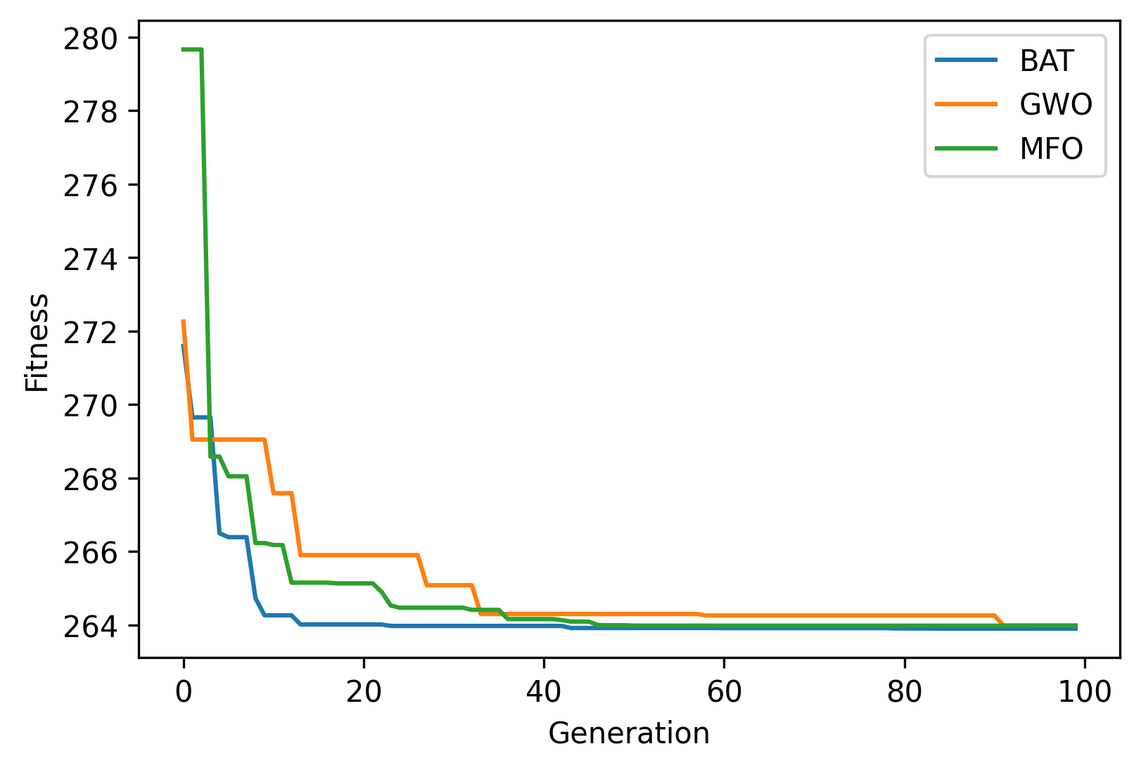
plt.figure()
plt.plot(bat_hist['global_fitness'], label = 'BAT')
plt.plot(gwo_hist['fitness'], label = 'GWO')
plt.plot(mfo_hist['global_fitness'], label = 'MFO')
plt.legend()
plt.xlabel('Generation')
plt.ylabel('Fitness')
plt.savefig('TBT_fitness.png',format='png', dpi=300, bbox_inches="tight")
plt.show()
6.4. Results
A summary of the results for the three differents methods is shown below with the best \((x_1, x_2)\) and \(y=f(x)\) (minimum volume).
------------------------ BAT Summary --------------------------
Best fitness (y) found: 263.90446934840577
Best individual (x) found: [0.79190302 0.39920471]
--------------------------------------------------------------
------------------------ GWO Summary --------------------------
Best fitness (y) found: 263.99180199625886
Best individual (x) found: [0.78831222 0.41023435]
--------------------------------------------------------------
------------------------ MFO Summary --------------------------
Best fitness (y) found: 263.9847325242824
Best individual (x) found: [0.77788022 0.4396698 ]
--------------------------------------------------------------