7. Example 7: Pressure Vessel Design
Example of solving the constrained engineering optimization problem “Pressure vessel design” using NEORL with the HHO, ES, PESA, and BAT algorithms to demonstrate compatibility with mixed discrete-continuous space.
7.1. Summary
Algorithms: HHO, ES, PESA, and BAT
Type: Mixed discrete-continuous, Single-objective, Constrained
Field: Mechanical Engineering
7.2. Problem Description
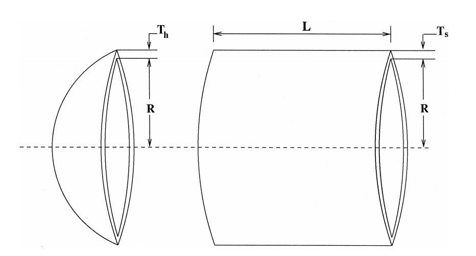
The pressure vessel design is an engineering optimization problem with the objective to evaluate the optimal thickness of shell (\(T_s = x_1\)), thickness of head (\(T_h = x_2\)), inner radius (\(R = x_3\)), and length of shell (\(L = x_4\)) such that the total cost of material, forming, and welding is minimized accounting for 4 constraints. \(T_s\) and \(T_h\) are integer multiples of 0.0625 in., which are the available thicknesses of rolled steel plates, and R and L are continuous. The figure below shows the dimensions of the pressure vessel structure.
The equation for the cost of the pressure vessel is
subject to 4 constraints
where \(0.0625 \leq x_1 \leq 6.1875\) (with step of 0.0625), \(0.0625 \leq x_2 \leq 6.1875\) (with step of 0.0625), \(10 \leq x_3 \leq 200\), and \(10 \leq x_4 \leq 200\).
7.3. NEORL script
########################
# Import Packages
########################

from neorl import HHO, ES, PESA, BAT
import math
import matplotlib.pyplot as plt

#############################
# Define Vessel Function
#(Mixed discrete/continuous)
#############################
def Vessel(individual):
    """
    Pressure vesssel design
    x1: thickness (d1)  --> discrete value multiple of 0.0625 in
    x2: thickness of the heads (d1) ---> discrete value multiple of 0.0625 in
    x3: inner radius (r)  ---> cont. value between [10, 200]
    x4: length (L)  ---> cont. value between [10, 200]
    """
    x=individual.copy()
    x[0] *= 0.0625   #convert d1 to "in"
    x[1] *= 0.0625   #convert d2 to "in"

    y = 0.6224*x[0]*x[2]*x[3]+1.7781*x[1]*x[2]**2+3.1661*x[0]**2*x[3]+19.84*x[0]**2*x[2];

    g1 = -x[0]+0.0193*x[2];
    g2 = -x[1]+0.00954*x[2];
    g3 = -math.pi*x[2]**2*x[3]-(4/3)*math.pi*x[2]**3 + 1296000;
    g4 = x[3]-240;
    g=[g1,g2,g3,g4]

    phi=sum(max(item,0) for item in g)
    eps=1e-5 #tolerance to escape the constraint region
    penality=1e7 #large penality to add if constraints are violated

    if phi > eps:
        fitness=phi+penality
    else:
        fitness=y
    return fitness


bounds = {}
bounds['x1'] = ['int', 1, 99]
bounds['x2'] = ['int', 1, 99]
bounds['x3'] = ['float', 10, 200]
bounds['x4'] = ['float', 10, 200]

########################
# Setup and evolute HHO
########################

hho = HHO(mode='min', bounds=bounds, fit=Vessel, nhawks=30,
                  int_transform='minmax', ncores=1, seed=1)
x_hho, y_hho, hho_hist=hho.evolute(ngen=200, verbose=False)
assert Vessel(x_hho) == y_hho

########################
# Setup and evolute ES
########################
es = ES(mode='min', fit=Vessel, cxmode='cx2point', bounds=bounds,
                 lambda_=60, mu=30, cxpb=0.7, mutpb=0.2, seed=1)
x_es, y_es, es_hist=es.evolute(ngen=200, verbose=False)
assert Vessel(x_es) == y_es

########################
# Setup and evolute PESA
########################
pesa=PESA(mode='min', bounds=bounds, fit=Vessel, npop=60, mu=30, alpha_init=0.1,
          alpha_end=1.0, cxpb=0.7, mutpb=0.2, alpha_backdoor=0.15, seed=1)
x_pesa, y_pesa, pesa_hist=pesa.evolute(ngen=200, verbose=False)
assert Vessel(x_pesa) == y_pesa

########################
# Setup and evolute BAT
########################
bat=BAT(mode='min', bounds=bounds, fit=Vessel, nbats=50, fmin = 0 , fmax = 1,
        A=0.5, r0=0.5, levy = True, seed = 1, ncores=1)
x_bat, y_bat, bat_hist=bat.evolute(ngen=200, verbose=1)
assert Vessel(x_bat) == y_bat

########################
# Plotting
########################

plt.figure()
plt.plot(hho_hist['global_fitness'], label='HHO')
plt.plot(es_hist['global_fitness'], label='ES')
plt.plot(pesa_hist, label='PESA')
plt.plot(bat_hist['global_fitness'], label='BAT')
plt.xlabel('Generation')
plt.ylabel('Fitness')
#plt.ylim([0,10000]) #zoom in
plt.legend()
plt.savefig('ex7_pv_fitness.png',format='png', dpi=300, bbox_inches="tight")
plt.show()

########################
# Comparison
########################

print('---Best HHO Results---')
print(x_hho)
print(y_hho)
print('---Best ES Results---')
print(x_es)
print(y_es)
print('---Best PESA Results---')
print(x_pesa)
print(y_pesa)
print('---Best BAT Results---')
print(x_bat)
print(y_bat)
7.4. Results
A summary of the results is shown below with the best \((x_1, x_2, x_3, x_4)\) and \(y=f(x)\) (minimum vessel cost). PESA seems to be the best algorithm in this case.
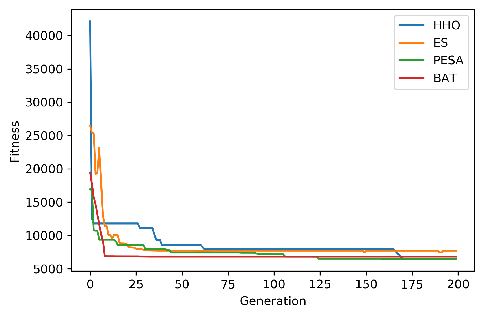
------------------------ HHO Summary --------------------------
Function: Vessel
Best fitness (y) found: 6450.086928941204
Best individual (x) found: [16.          8.         51.38667573 87.7107088 ]
--------------------------------------------------------------
------------------------ ES Summary --------------------------
Best fitness (y) found: 7440.247037114203
Best individual (x) found: [19, 10, 59.20709018618041, 39.15211859223507]
--------------------------------------------------------------
------------------------ PESA Summary --------------------------
Best fitness (y) found: 6446.821261696037
Best individual (x) found: [16, 8, 51.45490215425688, 87.29635265232538]
--------------------------------------------------------------
------------------------ BAT Summary --------------------------
Best fitness (y) found: 6820.372175171242
Best individual (x) found: [18.          9.         58.29066654 43.68984579]
--------------------------------------------------------------